Predicting Love at First 4 Minutes

Early into quarantine this year, I found myself addicted to the Netflix show, Love is Blind. The basic premise of the show is that a group of men and women participate in a “pod” experiment where they “date” with the hopes of getting engaged, without ever seeing the person! It’s wild and if you haven’t watched it yet, I highly recommend binging it!

Upon further reflection, I realized the concept of love at first sight is saturated in pop culture television and movies. Shows like The Bachelor, The Bachelorette, and Married at First Sight all capitalize on our fascination with the topic. I began to wonder if I could predict love at first sight and if so, what might be good predictors.

Methodology

In order to break this problem down further, I decided to see if I could predict love in the first 4 minutes of meeting. I used the Speed Dating Experiment data from Kaggle. The dataset includes information from 551 (presumptively) heterosexual men and women who attended 21 different speed dating events from 2002-2004. I found the dataset to be incredibly interesting! Each participant had between 5 and 22 rows of data, depending on the size of the speed dating event.

In order to examine love in 4 minutes at a deeper level, I built 2 separate models to fit 2 different targets. First, I set out to predict a match in a round of speed dating. Then I tried to predict a follow-up date after the speed dating event.

Matching in a Round of Speed Dating

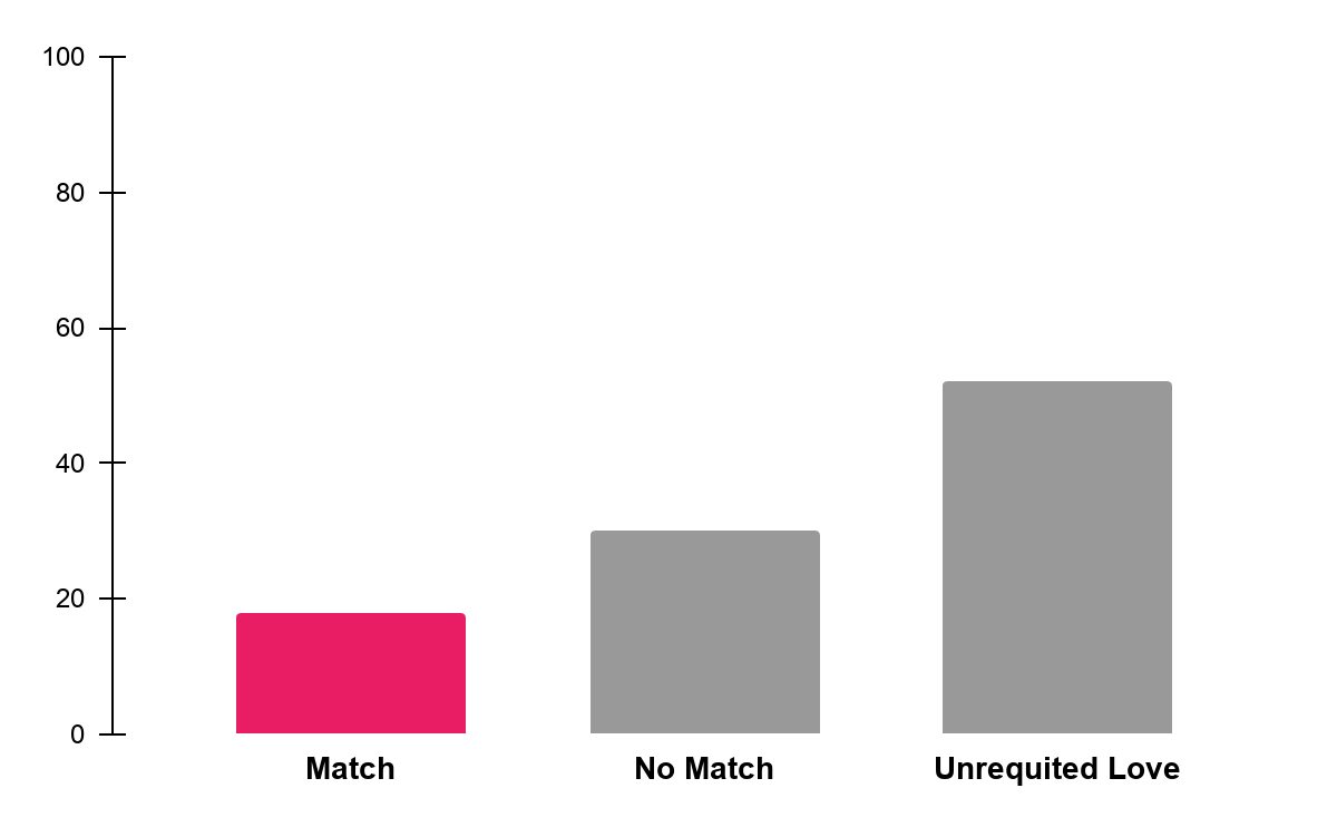
Figure 1: Percentage of each round ending in a match

There were 5,456 four-minute rounds of dates in the data. Quite surprisingly, only 18% of the rounds ended in a match. A match is when a participant and the date both decide “yes” on their scorecard. While I assumed speed dating would be challenging, I was surprised that matches were so low! More surprisingly though, 52% of the rounds ended in unrequited love, where one person said “yes” and the other said “no”. I’ve been married for nearly 4 years, and this data really brought me back to how challenging dating can be.

During each round of speed dating, each participant rated their date on various attributes on a scale of 1-10 (1 = lowest score, 10 = highest score). The attributes included attractive, sincere, intelligent, fun, ambitious, shared interests/hobbies, how much you like the person overall, how probable it is that they will say yes for you, and whether or not you’ve met the person before. Additionally, I did some feature engineering and created an in-sync feature which was the sum of the absolute value of ratings differences between you and your partner on each attribute in a round. For example, if a participant rated their date as a 5 for “Attractive” and the date rated the participant a 9, the absolute value of the difference is 4.

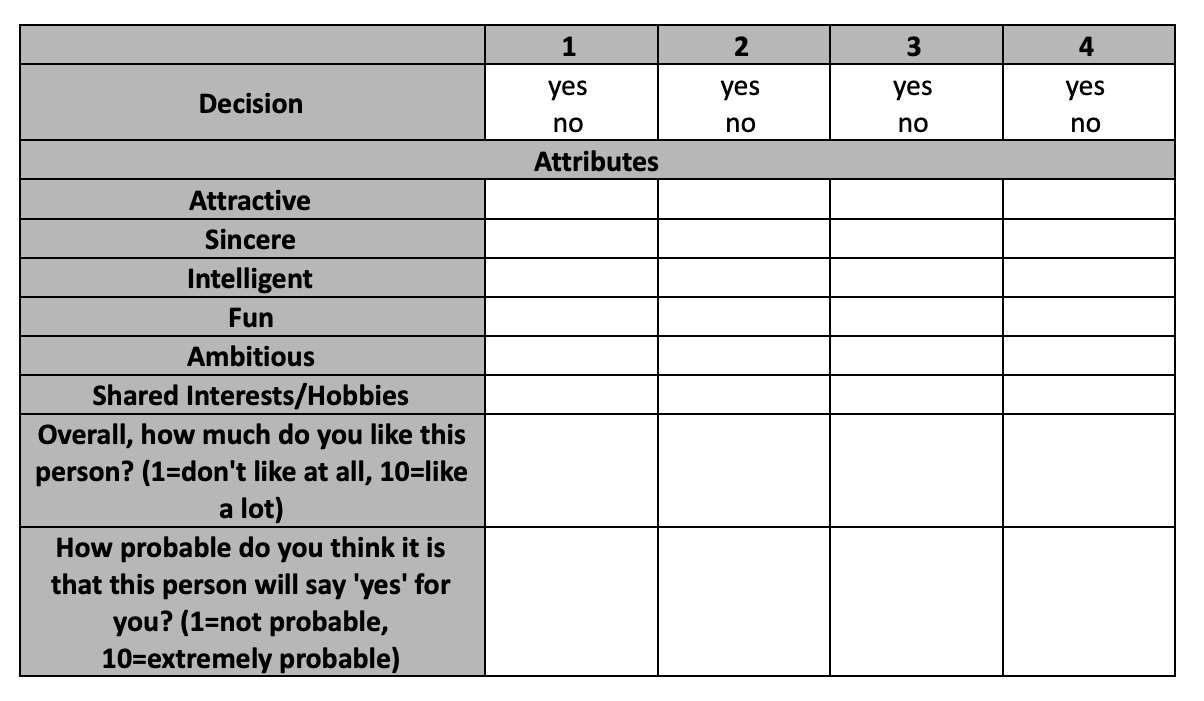
Figure 2: Sample scorecard from speed dating event

I tried a number of models to optimize for ROC/AUC. Ultimately, I chose a Logistic Regression model because it optimized ROC/AUC and provided opportunities for interpretation.

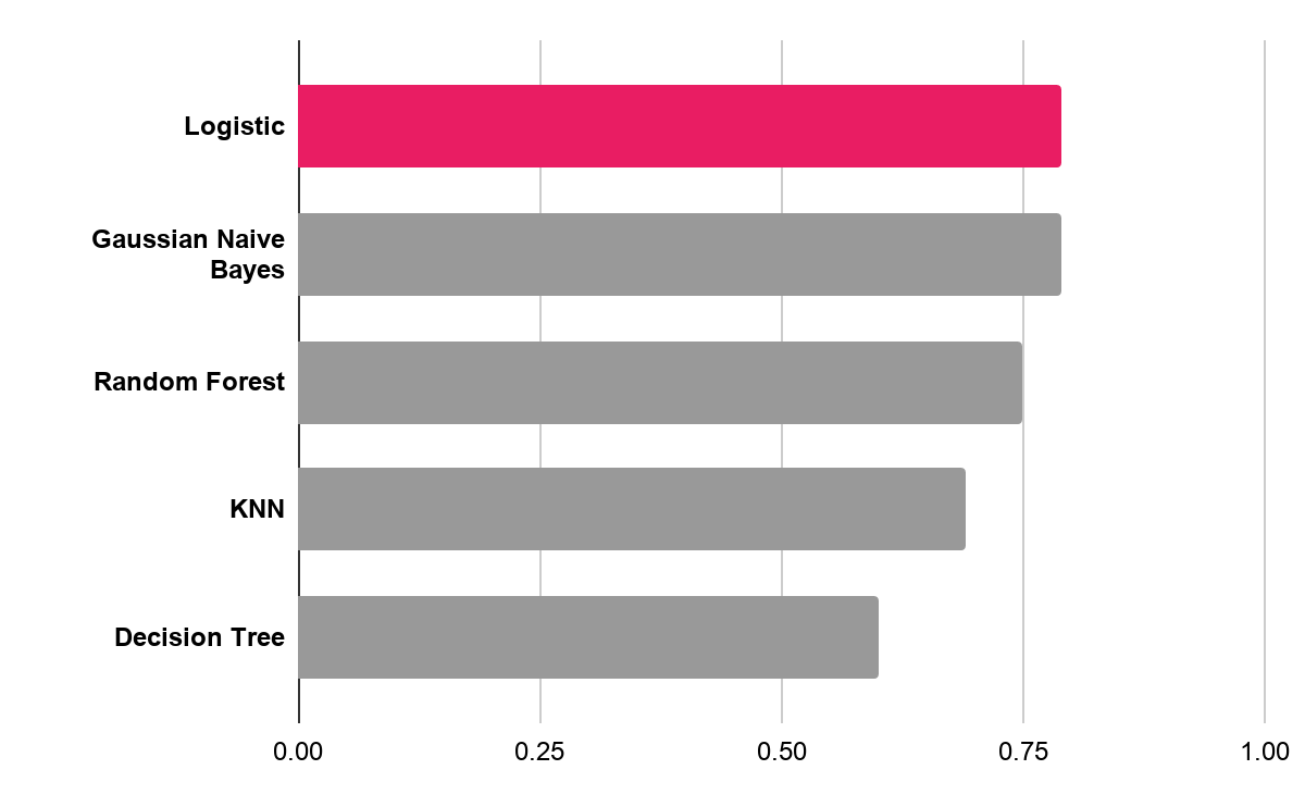
Figure 3: A logistic regression model was chosen because it provided the highest ROC AUC score and allowed for interpretation of coefficients

I was able to optimize ROC/AUC at 0.79 which means the model was able to account for some of the separation between match or not (even though accuracy performed on par with what would be expected from a dummy model). I tried various over/under sampling methods and SMOTE, but found this didn’t improve my results and added unnecessary complexity. I chose to optimize for ROC AUC for this model, so those who might potentially use the model in the future have the ability to choose their tolerance to false positives (i.e. predict a match, but it doesn’t happen) because people have their own dating baggage and therefore, might want to change their tolerance levels for disappointing results.

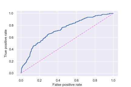
Figure 4: The ROC AUC graph for the final model's performance

Since this was a logistic regression model, I was excited to be able to dig into the impact of the features on the odds of matching. In the table below, you’ll see how much increasing each score changes the odds of matching. Most notably, how much you initially just “like” a person has a sizable increase on your odds. This makes intuitive sense, although it’s not necessarily the most helpful in terms of tangible advice for people who are dating. Additionally, while some of the other ratings themselves didn’t improve the model much, the sum of the absolute value of the ratings differences did. This somewhat contradicts the popular notion that opposites attract and should perhaps be revised to “partners who similarly perceive each other” attract.

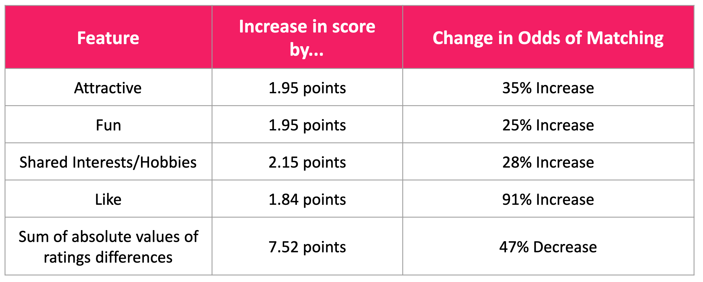
Figure 5: A breakdown of the impact of each feature on predicting the odds of a match

Predicting a Date After Speed Dating

Switching gears a bit, I wanted to dig in deeper to see which participants ended up going on a date after speed dating. This was a much smaller dataset because it was reliant on participants who submitted a follow-up survey after the event. Out of the original 551 participants, 223 completed the follow-up survey. But out of the 223 who completed the survey, 36% had a date. This number was actually higher than I was expecting; however, it’s worth noting that 328 of the original participants weren’t included in this! And it’s likely the people who didn’t return the survey didn’t go on a date afterwards. But acknowledging this, I’m going to look at individual participant information to see if I can predict who went on a date.

On the night of the event, participants were asked to fill out questionnaires about a lot of information. I grouped this information into 4 categories: interests, beliefs, lifestyle, and self-perception. The questions in the interests, beliefs and self-perception categories had participants rate themselves on a scale of 1-10 (1 = not interested/lowest value, 10 = highly interested/highest value). The scale for the lifestyle questions was out of 7 and a score of 1 indicated a high level of going out (several times per week), while a score of 7 indicated a low level of going out (almost never).

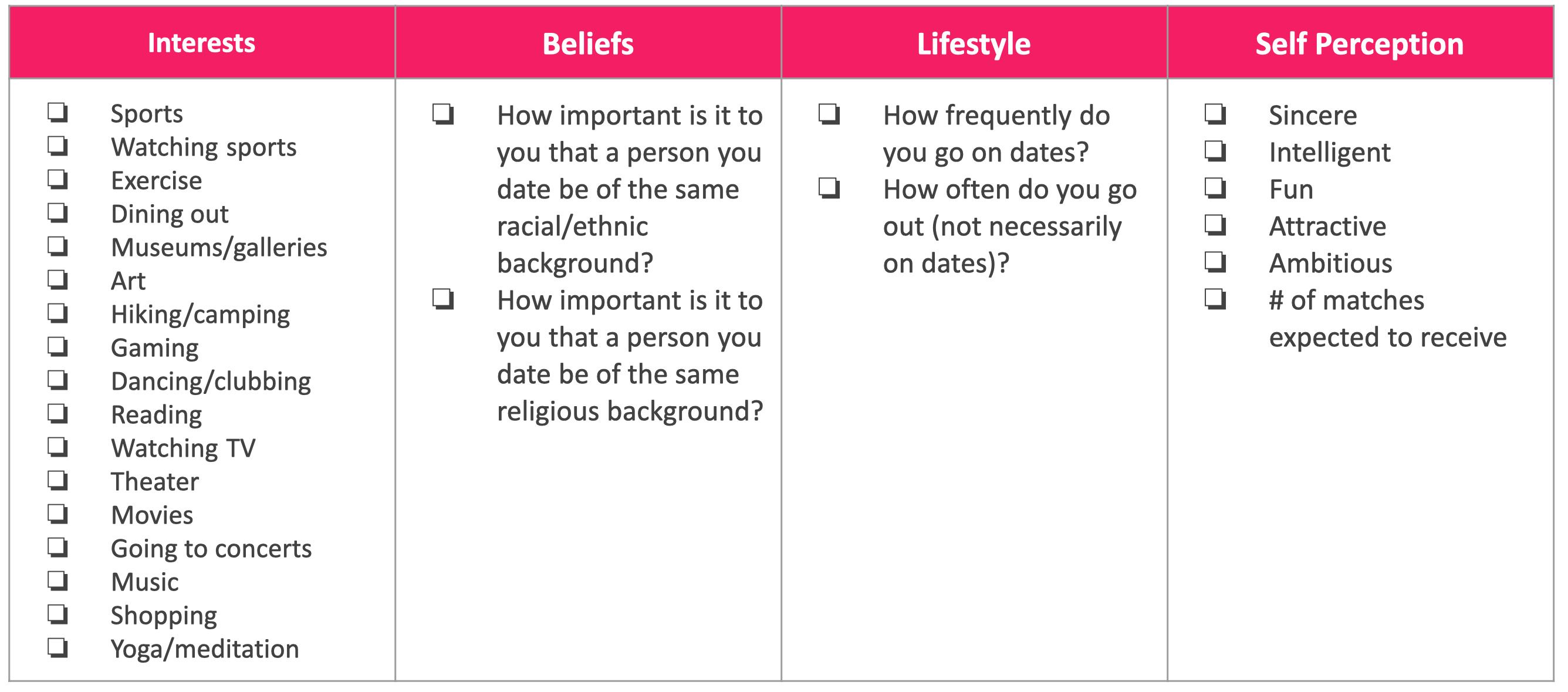
Figure 6: Questions asked of participants by category

Due to the small sample size and large number of features, I chose a Random Forest model and again worked to optimize ROC AUC for the same reasons as were previously stated. I chose a small number of features from the original questionnaire, but I found a lot more success when I did feature engineering to bucket by similar types of questions. For example, I bucketed participant responses to interests in watching TV, watching sports on TV and gaming into a broader category called “TV Oriented Activities”. You can see a visual of my engineered features below.

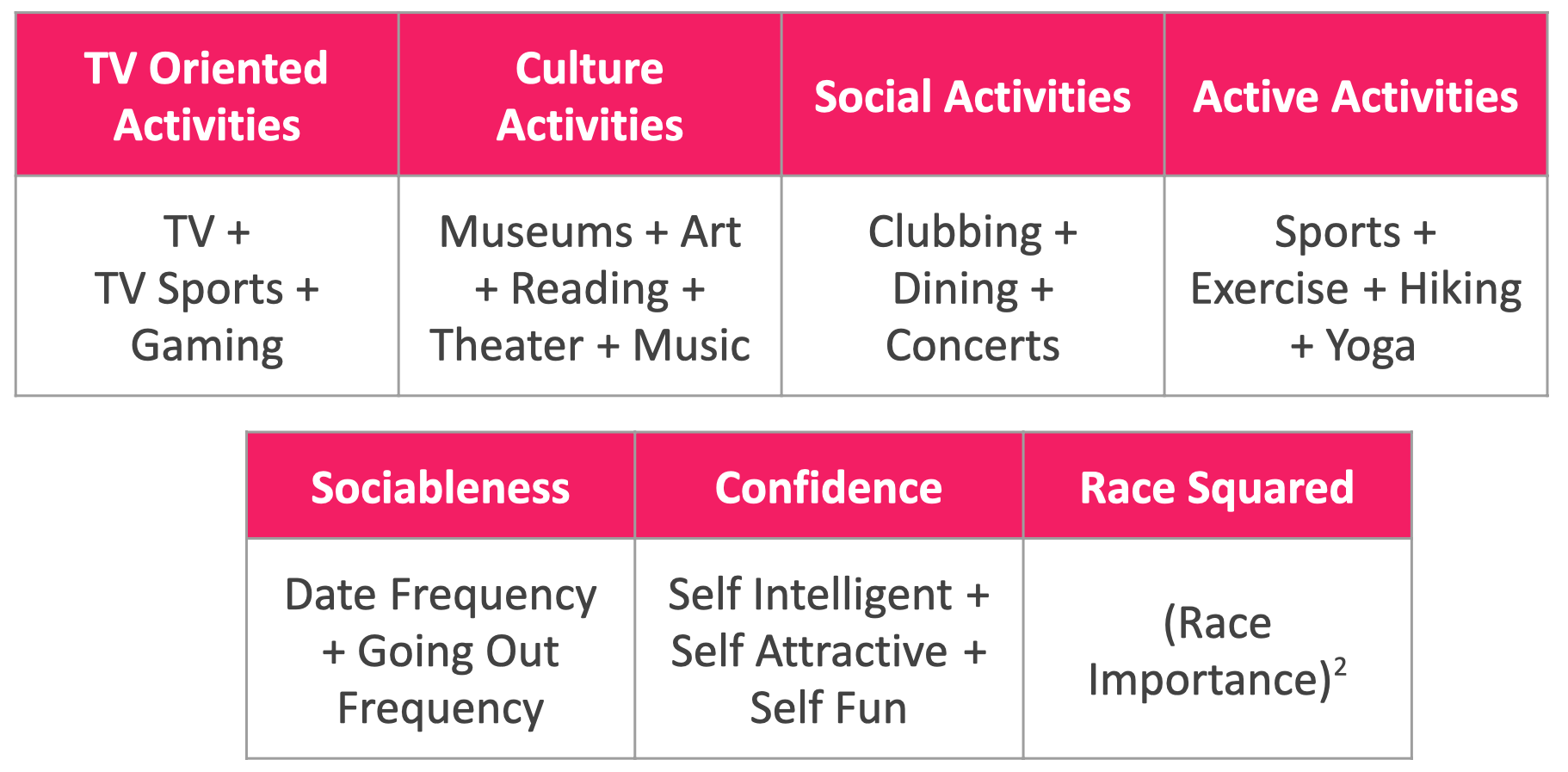
Figure 7: Categories of engineered features

This model did not have nearly as much success as my previous one, but I was able to optimize ROC AUC at 0.65. My model missed a lot of instances where people actually had dates, as evidenced by my confusion matrix below. I believe my model was limited by the relatively small sample size, and it appears that predicting a date is more complex than the features I included in my model!

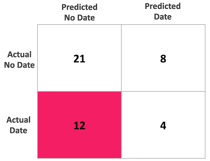
Figure 8: Confusion matrix highlighting the high amount of false negatives in the model

I had to include a lot of features in this model to even be able to optimize at the level I was able to, so I want to zoom in on a few of the most impactful features. Using Scikit-Learn’s Random Forest feature importance attribute and the rfpimp library’s permutation feature importance, I found that TV oriented activities, culture activities, active activities, and confidence were in the top 5 of both lists. I was surprised by a few of these features being so impactful! I didn’t expect Culture Activities to be rated lower on participants who had a date (I expected to see the opposite effect) and I was surprised that Active Activities was so impactful. However, in hindsight Active Activities makes sense given the impact of endorphins on mental health and perhaps that had a confounding effect on confidence/self-perception. One feature that I was particularly surprised to not see at the top of the most impactful features was the rating for the importance of race. In trying out various models and features, I found that when race importance wasn’t included in the model, the model performed significantly worse on the cross validation.

Local Flask App

I created a Flask App for users to enter information in and the app will predict whether they would have a date after a speed dating event. Below you’ll see a video of my app in action where I input feature scores from an actual participant in my test set to see how well my model predicted whether they would have a date! In this example, my model didn’t do too bad!

Figure 9: Demonstration of local flask model

Conclusions

If there’s one thing I took away from this, it’s that predicting human behavior around love and attraction is complex! My models had varying degrees of success and in all honesty, I think that’s a good thing! Love looks different for everyone and even though our algorithms might be complex, it’s still challenging to predict human behavior.

However, if you are dating and want some tangible conclusions from my results, I want to highlight the importance of first impressions! The more similar yours and a date’s perception of each other, the greater your odds of matching with that person. Additionally, the more you initially like a person, the greater your odds of matching are.

You can check out my code for my project on my Github.